Using Machine Learning components in critical systems requires a sound safety concept and the ability to argue and prove that the risk of the considered system is acceptably low. In our previous blog post (Dealing with uncertainties of Machine Learning components (Part 1), we discussed an approach using statistical distance measures for uncertainty estimation, one potential building block in a comprehensive safety concept. We demonstrated the effectiveness of the approach to gauge contextual relevance during runtime based on two example use cases, traffic sign recognition and person detection. In this post, we further extend the presented approach to include a context uncertainty estimation metric. Similar to the previous post of this series, we also demonstrate context uncertainty on two examples: German traffic sign recognition and person detection.

Using statistical distance measures for evaluating scope compliance at runtime (Part 2)

In the previous blog post, we motivated the crucial challenges of monitoring systems with Machine Learning components to ensure their reliability, safety, and effectiveness. In high-stakes environments such as healthcare, autonomous driving, industrial control, and financial systems, the consequences of model failures or inaccuracies can be severe, including risks to human life, significant financial loss, or operational disruptions.

Continuous monitoring allows detecting anomalies, performance degradation, and deviations from expected behavior in real time.

Monitoring approaches can help to identify issues such as data drift, where the statistical properties of the input data change over time, potentially leading to reduced model accuracy. Regular monitoring also aids in detecting biases, ensuring compliance with regulatory standards, and maintaining ethical standards by preventing discriminatory outcomes. By implementing adequate monitoring systems, organizations can trigger timely interventions such as model retraining, parameter adjustments, or even rollback to previous versions, thereby mitigating risks and maintaining the integrity and trustworthiness of critical systems.

In the last blog post, we addressed uncertainties arising from environmental factors. We proposed a statistical distance-based method to effectively identify contextual relevance during runtime. We further illustrated its working principle with two realistic examples. In this post, we expand on that by demonstrating how our approach can be used to quantitatively obtain scope compliance uncertainty by using the proposed Scope Compliance Uncertainty Metric (SCUE) (Farhad, Sorokos, Akram, & Aslansefat, 2024) for runtime use.

Example: Traffic sign recognition

For the demonstration, we again take the example of traffic sign recognition from Part 1 of this series of blog posts. In that post, we used the example to demonstrate the working principle of SafeML. The next step is to put this principle to use and build a Scope Compliance Uncertainty Estimate (SCUE). The algorithm for this is illustrated in the figure below.

Scope compliance uncertainty estimate algorithm: Fraunhofer IESE – Algorithm describing Scope compliance uncertainty estimate — Figure 1: Algorithm for Scope Compliance Uncertainty Estimate (SCUE)

To build the uncertainty estimator function in the design phase, we selected a sub-sample of our dataset. We then created a dataset “representative dataset” out of it. For this example, we used the German Traffic Sign Recognition Benchmark (GTSRB) dataset (Stallkamp, Schlipsing, Salmen, & Igel, 2011).

Calibration data

The calibration set was curated using the data from the test set of the desired application. The purpose of the calibration set is to establish a subset of data with decreasing performance (performance could be accuracy, mean-squared error, etc.). We achieved this by selecting 50% of the total data of the GTSRB dataset, with the samples selected randomly. Out of the selected data, we corrupted the first 75% with corruption type 1 (for example, Gaussian blur) and the last 75% with corruption type 2 (for example, fog). This led to an overlapping set containing 50% of the data, which in turn was corrupted using both type 1 and type 2 corruptions. Regarding the corruptions, we made use of image corruptions as introduced by (Michaelis, et al., 2019). The schematic representation of the process is shown below.

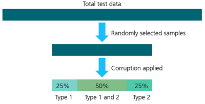
Distribution of subsets: Fraunhofer IESE – distribution of subsets for building scope compliance uncertainty estimate — Figure 2: Distribution of subsets for building a Scope Compliance Uncertainty Estimate

For the inference, we used the AlexNet model (Krizhevsky, Sutskever, & Hinton, 2023). We obtained a window of batches with decreasing performance (in this case, accuracy). The number of batches was selected to be 1500, with 50 samples in each batch.

Scope Compliance Uncertainty Estimate (SCUE)

To compute the Scope Compliance Uncertainty Estimate, we used regression analysis to fit a polynomial curve between the distance measured (Wasserstein, Kolmogrov-Smirnov, etc.) and the performance (inaccuracy, mean-squared error, etc.). For ease of computation, we also used Principal Component Analysis (PCA) on the penultimate layer and extracted the principal components.

Runtime execution is achieved by using Principal Component Analysis (PCA), a statistical technique used for dimensionality reduction while preserving as much variability as possible in a dataset.

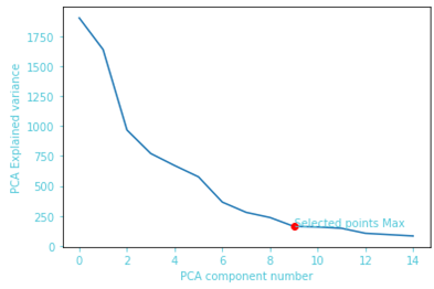
This transforms the original variables into a new set of uncorrelated variables called principal components, which are ordered by the amount of variance they capture from the data. The first principal component captures the maximum variance, followed by the second principal component, and so on. This transformation is achieved by finding the eigenvectors and eigenvalues of the covariance matrix of the data, where the eigenvectors represent the directions of maximum variance, and the eigenvalues denote the magnitude of this variance. By projecting the data onto these principal components, PCA reduces the dimensionality of the dataset, simplifying it while retaining its essential patterns and structures. We automatically selected the number of components that explain at least 85% of the total variance in the data. The graph below shows this process of automatically selecting the principal components.

Pricipal component analysis: Fraunhofer IESE – Automatically selecting number of components in PCA for GTSRB — Figure 3: Automatically selecting the number of components in PCA for traffic sign detection

Computing Statistical Distance Dissimilarity

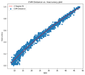
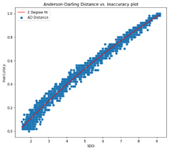
We then computed the SDD, i.e., Statistical Distance Dissimilarity (from Part 1 of this blog series) between the window of batches and the training data. We observed that the statistical distance-based estimators are consistent in ensuring that the correlation between the measured SDD and the observed performance (inaccuracy) behaves as desired. This means that the performance decreases with increasing SDD. The figure below shows the correlation on a second-degree polynomial curve that is fitted between the SDD obtained and the performance of the model recorded on the batch.

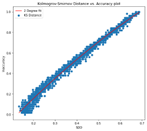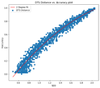The fit polynomial curve is used as a function of context uncertainty. The parameters are saved and are loaded for runtime use.

Runtime demo using SVHN

To demonstrate how context uncertainty be used at runtime, we used a dataset similar to the GTSRB dataset, called the Street View House Numbers (SVHN) dataset (Netzer et al., 2011). SVHN consists of over 600,000 labeled digits extracted from images of house numbers captured by Google Street View. Each image in the dataset contains a single digit (0-9), with annotations providing the digit label, bounding box coordinates, and the original image. Similar to GTSRB, SVHN has variability in digit appearance, lighting conditions, and background clutter, making it an excellent benchmark for evaluating the robustness and accuracy of digit recognition algorithms. The dataset is widely used in both academic research and practical applications for its relevance to real-world scenarios and its comprehensive annotations. The comparison below shows how the SVHN can be used as perfect out-of-domain (ODD) data for this example.

GTSRB Sample	SVHN Sample

For the sake of consistency, the images from the SVHN and GTSRB datasets were cropped to a size of 32*32. The table below shows the results of the SCUE values obtained on the samples from the SVHN dataset. As seen from the table, the polynomial curve successfully identified the SVHN as an OOD dataset.

Sample batch	SCUE - GTSRB	SCUE - SVHN
0	0.000	0.91
1	0.000	0.88
2	0.000	0.94
3	0.092	0.90
4	0.000	0.95
5	0.112	0.90
6	0.004	0.97
7	0.000	0.99
8	0.000	0.98
9	0.000	1.00

Example: Person detection

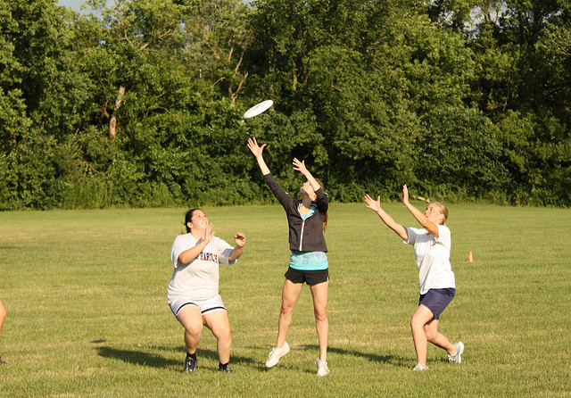
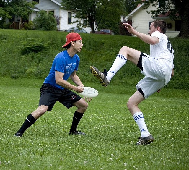
Let us further evaluate the method using a person detection example. The methodology employed is similar to the previous example of traffic sign recognition. In addition, we used the YOLO (Redmon & Farhadi, 2018) model trained on the COCO (Lin et al., 2014) dataset for person detection. We considered the CityScape (Cordts, et al., 2016) dataset to be out-of-domain data. The table below shows some samples from the COCO and the CityScape datasets.

COCO Sample	CityScape Sample

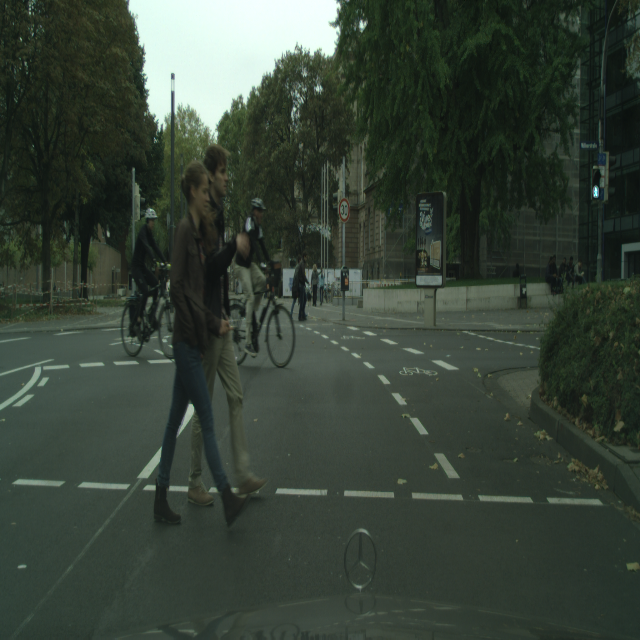Similar to traffic sign recognition, the table below shows the SCUE values obtained for in-domain and out-of-domain data. The values clearly indicate a distinction between the COCO and the CityScape datasets. Since the two datasets have a lot of similarities, it can be seen that the SCUE values are not as high for CityScape (compared to COCO) as they were for SVHN (compared to GTSRB).

Sample batch	SCUE - COCO	SCUE - CityScape
0	0.034	0.439
1	0.045	0.466
2	0.149	0.436
3	0.071	0.436
4	0.031	0.450
5	0.152	0.446
6	0.012	0.434
7	0.023	0.440
8	0.017	0.450
9	0.055	0.439

Conclusion

The previous blog post of this series demonstrated the principle of using Statistical Distance-based Dissimilarity (SDD) to obtain contextual relevance. In this post, we expanded on that to demonstrate how this principle can be tailored to obtain a scope compliance uncertainty metric at runtime. We demonstrated it using traffic sign recognition and person detection examples. If you would like to learn more and try it out yourself, we have made the demo available for public use. If you are interested in the topic or have any questions/comments, please feel free to contact us.

References

Cordts, M., Omran, M., Ramos, S., Rehfeld, T., Enzweiler, M., Benenson, R., . . . Schiele, B. (2016). The Cityscapes Dataset for Semantic Urban Scene Understanding. Proc. of the IEEE Conference on Computer Vision and Pattern Recognition (CVPR).

Farhad, A.-H., Sorokos, I., Akram, M., & Aslansefat, K. (2024). Scope Compliance Uncertainty Estimate Through Statistical Distance. Future of Information and Communication Conference, (pp. 413-432).

Krizhevsky, A., Sutskever, I., & Hinton, G. (2023). ImageNet classification with deep convolutional neural networks (AlexNet) ImageNet classification with deep convolutional neural networks (AlexNet). Actorsfit. Com.

Lin, T.-Y., Maire, M., Belongie, S., Hays, J., Perona, P., Ramanan, D., . . . Zitnick, C. (2014). Microsoft coco: Common objects in context. Computer Vision–ECCV 2014: 13th European Conference, September 6-12, 2014, Proceedings, Part V 13. Zurich, Switzerland.

Michaelis, C., Mitzkus, B., Geirhos, R., Rusak, E., Bringmann, O., Ecker, A., . . . Brendel, W. (2019). Benchmarking Robustness in Object Detection: Autonomous Driving when Winter is Coming. arXiv preprint arXiv:1907.07484.

Netzer, Y., Wang, T., Coates, A., Bissacco, A., Wu, B., & Y. Ng, A. (2011). Reading Digits in Natural Images with Unsupervised Feature Learning. NIPS Workshop on Deep Learning and Unsupervised Feature Learning.

Redmon, J., & Farhadi, A. (2018). Yolov3: An incremental improvement. arXiv preprint arXiv:1804.02767.

Stallkamp , J., Schlipsing , M., Salmen , J., & Igel, C. (2011). The {G}erman {T}raffic {S}ign {R}ecognition {B}enchmark: A multi-class classification competition. IEEE International Joint Conference on Neural Networks, (pp. 1453-1460).